Welcome
Facial Recognition
using Neural
Networks

Introduction
Backpropagation, an abbreviation for "backward propagation of errors", is a common method of training artificial neural networks. From a desired output, the network learns from many inputs, similar to the way a child learns to identify a dog from examples of dogs.The NN explained here contains three layers. These are input, hidden, and output Layers. During the training phase, the training data is fed into to the input layer. The data is propagated to the hidden layer and then to the output layer. This is called the forward pass of the back propagation algorithm. In forward pass, each node in hidden layer gets input from all the nodes from input layer, which are multiplied with appropriate weights and then summed. The output of the hidden node is the nonlinear transformation of the resulting sum. Similarly each node in output layer gets input from all the nodes from hidden layer, which are multiplied with appropriate weights and then summed. The output of this node is the non-linear transformation of the resulting sum. The output values of the output layer are compared with the target output values. The target output values are those that we attempt to teach our network. The error between actual output values and target output values is calculated and propagated back toward hidden layer. This is called the backward pass of the back propagation algorithm. The error is used to update the connection strengths between nodes, i.e. weight matrices between input-hidden layers and hidden-output layers are updated. During the testing phase, no learning takes place i.e., weight matrices are not changed. Each test vector is fed into the input layer. The feed forward of the testing data is similar to the feed forward of the training data.
In this assignment we were required to write/design a 3-layer backpropagation neural network ourselves to solve a 10-class face classification problem. The training and testing samples for this problem were obtained from the ORL face database.
(http://www.cl.cam.ac.uk/research/dtg/attarchive/facedatabase.html)
Although there were 40 classes in this database we were to choose the first 10 classes for our usage in the first section 1. There were 10 samples for each class.
Research
Before the project was started a lot of research was done on matlab and its functions as this was the first assignment based entirely on matlab.
Functions
Concatenate strings horizontally
str=strcat(‘Good’,’morning’)
combinedStr=strcat(s1,s2,….,sN)
str =
Goodmorning
Create array of all zeros
X = zeros(n) returns an n-by-n matrix of zeros.
X = zeros(sz1,...,szN,classname) returns an sz1-by-...-by-szN array of zeros of data type classname.
Read image from graphics file
A = imread(filename, fmt) reads a grayscale or color image from the file specified by the string filename. If the file is not in the current folder, or in a folder on the MATLAB® path, specify the full pathname.
Format data into string
str = sprintf(formatSpec,A1,...,An) formats the data in arrays A1,...,An according to formatSpec in column order, and returns the results to string str.
Random numbers and arrays
Y = rand(m,n) or Y = rand([m n]) returns an m-by-n matrix of random entries.
2-D Discrete Cosine Transform
B = dct2(A,m,n) pads the matrix A with 0's to size m-by-n before transforming. If m or n is smaller than the corresponding dimension of A,dct2 truncates A.
Indexing Vectors
Let's start with the simple case of a vector and a single subscript. The vector is:
v = [16 5 9 4 2 11 7 14];
The subscript can be a single value:
v(3) % Extract the third element
ans = 9
Or the subscript can itself be another vector:
v([1 5 6]) % Extract the first, fifth, and sixth elements
ans = 16 2 11
The colon notation in MATLAB provides an easy way to extract a range of elements from v: v(3:7) % Extract the third through the seventh elements
ans = 9 4 2 11 7
Swap the two halves of v to make a new vector:
v2 = v([5:8 1:4]) % Extract and swap the halves of v
v2 = 2 11 7 14 16 5 9 4
Indexing Matrices with Two Subscripts
A(2,4) % Extract the element in row 2, column 4
A(2:4,1:2) % Extract row 2 to 4 and column 1 to 2.
A(3,:) % Extract third row
A(:,end) % Extract last column
Image Input Methods
Mainly two types of methods were looked into which are as follows
- Discrete cosine transform (DCT) is closely related to the discrete Fourier transform. It is a separable linear transformation; that is, the two-dimensional transform is equivalent to a one-dimensional DCT performed along a single dimension followed by a one-dimensional DCT in the other dimension.
- Eigenvector mean technique: This method uses principal component analysis to determine the most discriminant features between images of face. The reason this technique was not used is because it is more complex and requires additional m file to operate the command.
Methodology
The task required us to write a code in matlab which would solve a 10 class classification problem using backprobogation method of neural networks. A sample code was given to us which solves a simple XOR Gate problem.
Matlab recognizes images as pixels and each pixel has a color value (as shown in figure 1).
These pixel form a matrix of values which in our case is 112 X 92.To simplify our process complexity the images were rescaled to
1000 X 1 matrix. This way we can feed the pixel values as input elements of the Network. The images are then feed into the network for training process and the output /target matrix is defined. The output matrix contains only zeroes and ones.
The class number is defined by the location of the number of ones. The training process is then started and the network keeps updating the weights until the sum error reaches the tolerance value. After the training process a sample images is feed into the network. The trained weights of the network are feed into another algorithm which multiples the weights with their respective neurons and gives the output numbers of the image. The highest value of the matrix is found (variable ‘max’) along with its corresponding position (variable ‘index’). This matrix is then converted into zeroes and one (one at the max value number) and then compared with the target matrix .This procedure is repeated for 5 images of all the 10 classes. The number of pictures correctly classified is then calculated and thus the percentage accuracy.
The code for Section 1 task one is given in the appendix.
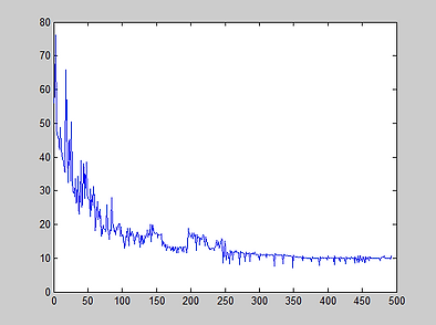
The Sum error was around 6-20% which is good error percentage. The accuracy percentage varied around 50 -75% which is quiet good as the number of input dimension (100) is considered it seems quite reasonable. If the input dimension was increased the process gets very slow and sometimes even hangs the computer
Percentage error vs Itterations
The code
TRAINING CODE
clc;
clear;
Input_dimension = 100;
number_of_classes=10;
input_images_per_class=5;
number_of_column =1;
Total_inputs=number_of_classes*input_images_per_class;
inputs = zeros(Total_inputs,Input_dimension) ;
for a= 1 : number_of_classes
for b= 1 :input_images_per_class
% Location of the files.
input_image = strcat('C:\Users\Murtaza Hassan\Desktop\Year 3\Neural networks\Neural Networks Project\s',sprintf('%d',a),'\',sprintf('%d',b),'.pgm');
% Storing the image.
stored_image = imread(input_image);
% Reshaping the image to respective dimension.
reshaped_image = dct2(stored_image,[Input_dimension,1]);
% Storing the image to the zero matrix.
inputs(number_of_column,:)=reshaped_image;
% Updating the number of coloumn for next image.
number_of_column =number_of_column+1;
end
end
% BACK PROPAGATION ALGORITHM
eta = 1;
alpha = 0.1;
tol = 0.5;
Q = Total_inputs ; %number of samples
n = Input_dimension; % number of input elements
q = 150; % number of output elements
p = 10; % number of classes
Iterate = 1;
D1=ones(1,input_images_per_class);
D0=zeros(1,input_images_per_class);
Wih = 2 * rand(n+1,q) - 1; %Input-hidden weight matrix
Whj = 2 * rand(q+1,p) - 1; %Hidden-Output weight matrix
DeltaWih = zeros(n+1,q); %Weight Change Matrix
DeltaWhj = zeros(q+1,p); %Weight Change Matrix
DeltaWihOld = zeros(n+1,q);
DeltaWhjOld = zeros(q+1,p);
Si = [ones(Q,1) inputs]; %input signals
D2 =[D1 D0 D0 D0 D0 D0 D0 D0 D0 D0
D0 D1 D0 D0 D0 D0 D0 D0 D0 D0
D0 D0 D1 D0 D0 D0 D0 D0 D0 D0
D0 D0 D0 D1 D0 D0 D0 D0 D0 D0
D0 D0 D0 D0 D1 D0 D0 D0 D0 D0
D0 D0 D0 D0 D0 D1 D0 D0 D0 D0
D0 D0 D0 D0 D0 D0 D1 D0 D0 D0
D0 D0 D0 D0 D0 D0 D0 D1 D0 D0
D0 D0 D0 D0 D0 D0 D0 D0 D1 D0
D0 D0 D0 D0 D0 D0 D0 D0 D0 D1];
D=transpose(D2); %Desired values
Sh = [1 zeros(1,q)]; %hidden Neural Signals
Sy = zeros(1,p); %output Neuron Signal
deltaO = zeros(1,p); %Error-slope product at output
deltaH = zeros(1,q+1); %Error-slope product at hidden
sumerror = 2*tol; %To get in to the loop
while (sumerror > tol) %iterate
sumerror = 0;
for k = 1:Q
Zh = Si(k,:) * Wih; %Hidden activations
Sh = [1 1./(1 + exp(-Zh))];
Yj = Sh * Whj;
Sy = 1./(1 + exp(-Yj));
Ek =D(k,:) - Sy;
deltaO = Ek .* Sy .* (1 - Sy);
for h = 1:q+1
DeltaWhj(h,:) = deltaO * Sh(h);
end
for h = 2:q+1
deltaH(h) = (deltaO * Whj(h,:)') * Sh(h) * (1-Sh(h));
end
for i= 1:n+1
DeltaWih(i,:) = deltaH(2:q+1) * Si(k,i);
end
Wih = Wih + eta * DeltaWih + alpha * DeltaWihOld;
Whj = Whj + eta * DeltaWhj + alpha * DeltaWhjOld;
DeltaWihOld = DeltaWih; %Store changes
DeltaWhjOld = DeltaWhj;
sumerror = sumerror + sum (Ek.^2); %Compute error
end
sumerror;
Iterate;
error (Iterate) = sumerror
plot (error);figure(gcf)
Iterate = Iterate + 1;
end
TESTING CODE
Total_inputs=50;
inputs = zeros(Total_inputs,Input_dimension) ;
number_of_column=1;
for a= 1 : number_of_classes
for b= 6 : 10
% Location of the files.
input_image = strcat('C:\Users\Murtaza Hassan\Desktop\Year 3\Neural networks\Neural Networks Project\s',sprintf('%d',a),'\',sprintf('%d',b),'.pgm');
% Storing the image.
stored_image = imread(input_image);
% Reshaping the image to respective dimension.
reshaped_image = dct2(stored_image,[Input_dimension,1]);
% Storing the image to the zero matrix.
inputs(number_of_column,:)=reshaped_image;
% Updating the number of coloumn for next image.
number_of_column =number_of_column+1;
end
end
% Output of Neural network for testing
Si = [ones(Total_inputs,1) inputs];
net_outputs = zeros(Total_inputs,number_of_classes);
for k = 1:Total_inputs
Zh = Si(k,:) * Wih; % Hidden activations
Sh = [1 1./(1 + exp(-Zh))]; % Hidden signals
Yj = Sh * Whj; % Output activations
Sy = 1./(1 + exp(-Yj)); % Output signals
net_outputs(k,:) = Sy;
end
test = vec2ind(net_outputs');
% test matrix
a = [1 1 1 1 1 2 2 2 2 2 3 3 3 3 3 4 4 4 4 4 5 5 5 5 5 6 6 6 6 6 7 7 7 7 7 8 8 8 8 8 9 9 9 9 9 10 10 10 10 10];
Number_of_pics_matched = sum(test == a); % check classification accuracy
Accuracy_percentage= 100*(Number_of_pics_matched/50)